
Developer's Development
3.3.21 [LLM] 자연어-이미지 멀티모달: CNN 개요 및 구조 본문
합성곱 신경망 (Convolutional Neural Network, CNN)
- CNN의 기본 개념
👉🏻 합성곱(Convolution)이란
이미지 처리에서 주변 필셀과의 가중합을 계산하여 특징을 추출하는 연산이다.
합성곱 신경망에서 합성곱 연산은 커널(또는 필터)을 사용하여 입력 데이터와의 내적을 수행한다.
합성곱 신경망의 구성 개요
- 합성곱 계층(Convolutional Layer): 필터(커널)를 이용하여 이미지의 특징을 추출
- 풀링 계층(Pooling Layer): 데이터의 크기를 줄이고 중요한 특징을 유지하여 연산량 감소
- 완전 연결 계층(Fully Connected Layer): 최종적으로 학습된 특징을 바탕으로 분류 또는 회귀 수행
- 배치 처리: 배치(Batch) 처리는 여러 개의 입력 데이터를 한 번에 연산하는 방식으로, 학습을 안정적으로 수행하고 연산 속도를 향상시킨다.
합성곱 신경망은 딥러닝의 한 분야로 이미지 인식과 처리에 주로 사용되는 인공신경망(ANN)의 한 종류이다.
이미지 분류, 객체 인식 및 탐지, 얼굴 인식, 의료 이미지 분석 등에 응용 가능하다.
[ 합성곱층의 필요성 ]
완전 연결 신경망(FCNN)은 이미지의 공간적 특성을 고려하지 않고 1차원 벡터로 변환하여 학습하므로, 지역적인 특징을 무시하고 연산량이 증가하는 문제가 발생한다. 이를 해결하기 위해 합성곱 신경망(CNN)이 도입되었다.
👉🏻 필터 & 특징 맵
1. 필터 (Filter)
- 합성곱 연산에서 사용하는 커널이다.
- 필터는 학습을 통해 최적의 값을 찾으며, 특정한 특징을 추출하는 역할을 한다.
2. 특징 맵 (Feature Map)
- 필터를 입력 데이터에 적용하여 얻은 출력이다.
- 입력 이미지에서 특정한 패턴이나 특징을 강조한다.
3. 필터와 특징 맵의 관계
- 여러 개의 필터를 사용하면 여러 개의 특징 맵이 생성된다.
- 각 필터는 다른 특징을 추출하도록 학습된다.
👉🏻 패딩 & 스트라이드
1. 패딩(Padding)
- 입력 데이터의 가장자리에 특정 값(보통 0)을 추가하여 출력 크기를 조정한다.
- 유형
- Valid Padding: 패딩을 사용하지 않아 출력 크기가 줄어든다.
- Same Padding: 출력 크기를 입력과 동일하게 유지하기 위해 패딩을 추가한다.
2. 스트라이드(Stride)
- 필터를 이동시키는 간격을 의미한다.
- 스트라이드 값이 클수록 출력 크기가 작아진다.
- 풀링 레이어
👉🏻 풀링(Pooling)이란
공간적 크기를 줄여 계산량을 감소시키고, 특징의 위치 변화에 대한 강건성을 높이는 연산이다.
👉🏻 풀링의 종류
1. 최대 풀링 (Max Pooling)
- 주어진 필터(영역 내)에서 가장 큰 값을 선택한다.
- 가장 중요한 특징을 유지하면서도 크기를 줄일 수 있다. (에지와 같은 중요한 특징을 강조)
- 경계 감지나 이미지의 강한 특징을 보존하는 데 유리하다.
2. 최소 풀링 (Min Pooling)
- 지정된 필터 크기 내에서 가장 작은 값을 선택하여 출력한다.
- 가장 어두운 픽셀이나 작은 값이 중요한 경우에 사용될 수 있다.
- 하지만 일반적인 CNN 모델에서는 거의 사용되지 않는다.
3. 평균 풀링 (Average Pooling)
- 필터(영역) 내의 모든 값을 평균 내어 출력한다.
- 전체적인 정보 보존이 필요할 때 유용하지만, 가장 두드러진 특징이 약해질 수 있다.
4. 글로벌 풀링 (Global Average Pooling)
- 전체 입력을 하나의 값으로 변환한다.
- 글로벌 최대 풀링 (Global Max Pooling): 전체 특징 맵에서 가장 큰 값을 반환한다.
- 글로벌 평균 풀링 (Global Average Pooling): 전체 값의 평균을 반환한다.
- 주로 CNN 마지막 단계에서 완전 연결층(FC Layer)을 제거하고 특징을 요약하는 데 사용된다.
(전체적인 흐름이나 배경 정보를 추출)
👉🏻 풀링의 효과
계산량 감소, 특징의 불변성 증가, 과적합 방지
- CNN의 구조와 동작
👉🏻 일반적인 CNN 구조
1. 합성곱 레이어 (Convlutional Layer): 특징을 추출하는 역할을 한다.
2. 활성화 함수(Activation Function): 비선형성을 도입하여 모델의 표현력을 높인다. ex) ReLU 함수
3. 풀링 레이어 (Pooling Layer): 공간적 크기를 줄여 계산 효율성을 높인다.
4. 완전 연결 레이어 (Fully Connected Layer): 추출된 특징을 기반으로 분류나 회귀를 수행한다.
👉🏻 CNN의 순전파 과정
1. 입력 이미지 전달: 모델의 입력으로 이미지 데이터를 받는다.
2. 합성곱 연산: 필터를 사용하여 특징 맵을 생성한다.
3. 활성화 함수 적용: 비선형 활성화 함수를 통해 특징 맵에 비선형성을 부여한다.
4. 풀링 연산: 풀링 레이어를 통해 공간적 크기를 축소한다.
5. 완전 연결 레이어: 1차원 벡터로 변환하여 최종 출력을 계산한다.
실습 (손글씨 숫자 예측 by MLP, colab)
from torchvision.datasets.mnist import MNIST	# 손글씨 숫자 데이터
from torchvision.transforms import ToTensor

train_data = MNIST(root='./', train=True, download=True, transform=ToTensor())
test_data = MNIST(root='./', train=False, download=True, transform=ToTensor())
# 받아온 데이터의 크기 확인
print(len(train_data), len(test_data))
print(train_data.data.shape)
"""
60000 10000
torch.Size([60000, 28, 28])
"""import matplotlib.pyplot as plt
plt.imshow(train_data.data[9])
plt.show()
from torch.utils.data.dataloader import DataLoader

train_loader = DataLoader(train_data, batch_size=64, shuffle=True)
test_loader = DataLoader(test_data, batch_size=64, shuffle=False)
import torch
device= 'cuda' if torch.cuda.is_available() else 'cpu'
device # 'cuda'# MLP 모델
import torch.nn as nn
class MLP(nn.Module):
def __init__(self):
super().__init__()
self.fc1 = nn.Linear(784, 128)
self.relu1 = nn.ReLU()
self.fc2 = nn.Linear(128, 64)
self.relu2 = nn.ReLU()
self.fc3 = nn.Linear(64, 10)
def forward(self, x):
x = x.view(x.size(0), -1) # [B, 1, 28, 28] -> [B, 784]
x = self.relu1(self.fc1(x))
x = self.relu2(self.fc2(x))
return self.fc3(x)
model = MLP().to(device)# 학습
from torch.optim.adam import Adam
learning_rate = 1e-3
optim = Adam(model.parameters(), lr=learning_rate)
for epoch in range(20):
for data, label in train_loader:
optim.zero_grad()
data = torch.reshape(data, (-1, 784)).to(device)
preds = model(data)
loss = nn.CrossEntropyLoss()(preds, label.to(device))
loss.backward()
optim.step()
print(f"Epoch: {epoch + 1}, Loss: {loss.item():.4f}") # Loss 들쭉날쭉함# 모델의 가중치 저장
torch.save(model.state_dict(), 'MNIST.pt')
# 모델 로드 (가중치 로드)
model.load_state_dict(torch.load('MNIST.pt', map_location=device
# 모델 예측 및 평가
correct = 0
with torch.no_grad():
for data, label in test_loader:
data = torch.reshape(data, (-1, 784)).to(device)
output = model(data)
preds = output.data.max(1)[1] # 최댓값을 가진 인덱스를 가져오도록
# preds = output.argmax(dim=1) # 위 코드와 같은 뜻
corr = preds.eq(label.to(device).data).sum().item()
correct += corr
print(f"Accuracy: {correct / len(test_data)}") # Accuracy: 0.9784 -> 꽤 높음!
실습 (Conv + Pool, colab)
💧 CNN 구조를 PyTorch 이용해서 간단하게 만들어보기
import torch
import torch.nn as nn
import torch.nn.functional as F
import torch.optim as optim

input_tensor = torch.randn(1, 1, 28, 28)    # (batch, channel, height, width) -> 흑백 이미지

conv = nn.Conv2d(
    in_channels=1,          # 입력 한장
    out_channels=4,       # 4개의 채널로 출력
    kernel_size=3,
    stride=1,
    padding="same"     # padding의 기본값은 valid
)

pool = nn.MaxPool2d(    # 풀링 레이어
    kernel_size=2,
    stride=2
)

output = F.relu(conv(input_tensor))
print(output.shape)

output = pool(output)
print(output.shape)
"""
torch.Size([1, 4, 28, 28])	# 4개의 특징 맵으로 4차원
torch.Size([1, 4, 14, 14])	# 반이 감소
"""

print(conv.weight.shape)
print(conv.bias.shape)
"""
torch.Size([4, 1, 3, 3])
torch.Size([4])
"""
- CNN Model
1. Feature Extraction Layer
2. Fully Connected (Classification) Layer
class CNNModel(nn.Module):
    def __init__(self):
        super().__init__()

        # 특성추출층
        self.conv1 = nn.Conv2d(1, 32, kernel_size=3, padding='same')
        self.conv2 = nn.Conv2d(32, 64, kernel_size=3, padding='valid')
        self.pool = nn.MaxPool2d(2, 2)

        # 완전연결층
        self.flatten = nn.Flatten()
        self.fc1 = nn.Linear(64 * 13 * 13, 100)
        self.fc2 = nn.Linear(100, 10)

    def forward(self, x):
        x = F.relu(self.conv1(x))
        x = F.relu(self.conv2(x))
        x = self.pool(x)
        x = self.flatten(x)
        x = F.relu(self.fc1(x))
        x = self.fc2(x)
        return x

model = CNNModel()
model
"""
CNNModel(
  (conv1): Conv2d(1, 32, kernel_size=(3, 3), stride=(1, 1), padding=same)
  (conv2): Conv2d(32, 64, kernel_size=(3, 3), stride=(1, 1), padding=valid)
  (pool): MaxPool2d(kernel_size=2, stride=2, padding=0, dilation=1, ceil_mode=False)
  (flatten): Flatten(start_dim=1, end_dim=-1)
  (fc1): Linear(in_features=10816, out_features=100, bias=True)
  (fc2): Linear(in_features=100, out_features=10, bias=True)
)
"""
!pip install torchsummaryfrom torchsummary import summary
summary(model, (1, 28, 28))
"""
----------------------------------------------------------------
Layer (type) Output Shape Param #
================================================================
Conv2d-1 [-1, 32, 28, 28] 320
Conv2d-2 [-1, 64, 26, 26] 18,496
MaxPool2d-3 [-1, 64, 13, 13] 0
Flatten-4 [-1, 10816] 0
Linear-5 [-1, 100] 1,081,700
Linear-6 [-1, 10] 1,010
================================================================
Total params: 1,101,526
Trainable params: 1,101,526
Non-trainable params: 0
----------------------------------------------------------------
Input size (MB): 0.00
Forward/backward pass size (MB): 0.69
Params size (MB): 4.20
Estimated Total Size (MB): 4.89
----------------------------------------------------------------
"""
실습 (Fashion MNIST (grayscale))
CNN: 흑백 FashionMNIST 데이터셋 활용
https://github.com/zalandoresearch/fashion-mnist
GitHub - zalandoresearch/fashion-mnist: A MNIST-like fashion product database. Benchmark
A MNIST-like fashion product database. Benchmark :point_down: - GitHub - zalandoresearch/fashion-mnist: A MNIST-like fashion product database. Benchmark
github.com
- 1. 데이터 로드
from torchvision import datasets

train_dataset = datasets.FashionMNIST(root='./', train=True, download=True)
test_dataset = datasets.FashionMNIST(root='./', train=False, download=True)

train_dataset, test_dataset
"""
(Dataset FashionMNIST
     Number of datapoints: 60000
     Root location: ./
     Split: Train,
 Dataset FashionMNIST
     Number of datapoints: 10000
     Root location: ./
     Split: Test)
"""

print(train_dataset[0])
print(train_dataset.data[0])	# 픽셀 단위로 해상도를
print(train_dataset.data.shape)	# torch.Size([60000, 28, 28])
# 전처리 (채널차원 추가 및 정규화)
train_images = train_dataset.data.unsqueeze(1) / 255.0 # 0~1
train_images = (train_images - 0.5) / 0.5 # -1~1
train_labels = train_dataset.targets.long()
test_images = test_dataset.data.unsqueeze(1) / 255.0
test_images = (test_images - 0.5) / 0.5
train_labels = test_dataset.targets.long()# 학습/검증 데이터셋 분할
from sklearn.model_selection import train_test_split
train_idx, val_idx = train_test_split(range(len(train_images)), test_size=0.15, random_state=42)
tr_images = train_images[train_idx]
tr_labels = train_labels[train_idx]
val_images = train_images[val_idx]
val_labels = train_labels[val_idx]
데이터 시각화
import numpy as np
import matplotlib.pyplot as plt

random_idx = np.random.choice(len(tr_images), 10, replace=False)
random_images = tr_images[random_idx]
random_labels = tr_labels[random_idx]

class_name = train_dataset.classes

plt.figure(figsize=(12, 6))
for i in range(10):
    plt.subplot(2, 5, i+1)

    img = random_images[i].squeeze()
    plt.imshow(img, cmap='gray')
    plt.title(f"Label: {class_name[random_labels[i]]}")
    plt.axis('off')

plt.tight_layout()
plt.show()
- 2. 모델 생성
import torch
import torch.nn as nn
import torch.nn.functional as F
import torch.optim as optim

class FashionMNISTCNN(nn.Module):
    def __init__(self):
        super().__init__()

        self.conv1 = nn.Conv2d(1, 32, kernel_size=3, padding='same')
        self.conv2 = nn.Conv2d(32, 64, kernel_size=3, padding='valid')
        self.pool = nn.MaxPool2d(2, 2)

        self.flatten = nn.Flatten()
        self.dropout1 = nn.Dropout(0.3)
        self.fc1 = nn.Linear(64 * 13 * 13, 100)
        self.dropout2 = nn.Dropout(0.2)
        self.fc2 = nn.Linear(100, 10)

    def forward(self, x):
        x = F.relu(self.conv1(x))
        x = F.relu(self.conv2(x))
        x = self.pool(x)

        x = self.flatten(x)
        x = self.dropout1(x)
        x = F.relu(self.fc1(x))
        x = self.dropout2(x)
        return self.fc2(x)

model = FashionMNISTCNN()
model
"""
FashionMNISTCNN(
  (conv1): Conv2d(1, 32, kernel_size=(3, 3), stride=(1, 1), padding=same)
  (conv2): Conv2d(32, 64, kernel_size=(3, 3), stride=(1, 1), padding=valid)
  (pool): MaxPool2d(kernel_size=2, stride=2, padding=0, dilation=1, ceil_mode=False)
  (flatten): Flatten(start_dim=1, end_dim=-1)
  (dropout1): Dropout(p=0.3, inplace=False)
  (fc1): Linear(in_features=10816, out_features=100, bias=True)
  (dropout2): Dropout(p=0.2, inplace=False)
  (fc2): Linear(in_features=100, out_features=10, bias=True)
)
"""
from torchsummary import summary
summary(model, (1, 28, 28), device="cpu")
"""
----------------------------------------------------------------
Layer (type) Output Shape Param #
================================================================
Conv2d-1 [-1, 32, 28, 28] 320
Conv2d-2 [-1, 64, 26, 26] 18,496
MaxPool2d-3 [-1, 64, 13, 13] 0
Flatten-4 [-1, 10816] 0
Dropout-5 [-1, 10816] 0
Linear-6 [-1, 100] 1,081,700
Dropout-7 [-1, 100] 0
Linear-8 [-1, 10] 1,010
================================================================
Total params: 1,101,526
Trainable params: 1,101,526
Non-trainable params: 0
----------------------------------------------------------------
Input size (MB): 0.00
Forward/backward pass size (MB): 0.77
Params size (MB): 4.20
Estimated Total Size (MB): 4.98
----------------------------------------------------------------
"""
- 3. 모델 학습
from torch.utils.data import TensorDataset, DataLoader

criterion = nn.CrossEntropyLoss()
optimizer = optim.Adam(model.parameters(), lr=0.001)

device = torch.device("cuda" if torch.cuda.is_available() else "cpu")
model = model.to(device)

batch_size = 128
train_dataset = TensorDataset(tr_images, tr_labels)
val_dataset = TensorDataset(val_images, val_labels)
test_dataset = TensorDataset(test_images, test_labels)

train_loader = DataLoader(train_dataset, batch_size=batch_size, shuffle=True)
val_loader = DataLoader(val_dataset, batch_size=batch_size, shuffle=False)
test_loader = DataLoader(test_dataset, batch_size=batch_size, shuffle=False)
history = {
"train_loss": [],
"train_acc": [],
"val_loss": [],
"val_acc": []
}
epochs = 30
for epoch in range(epochs):
model.train()
train_loss = 0.0
train_total = 0
train_correct = 0
for batch_idx, (images, labels) in enumerate(train_loader):
images, labels = images.to(device), labels.to(device)
optimizer.zero_grad()
outputs = model(images)
loss = criterion(outputs, labels)
loss.backward()
optimizer.step()
train_loss += loss.detach().cpu().item()
_, pred = torch.max(outputs.data, 1)
train_total += labels.size(0)
train_correct += (pred == labels).sum().detach().cpu().item()
model.eval()
val_loss = 0.0
val_total = 0
val_correct = 0
with torch.no_grad():
for batch_idx, (images, labels) in enumerate(val_loader):
images, labels = images.to(device), labels.to(device)
outputs = model(images)
loss = criterion(outputs, labels)
val_loss += loss.detach().cpu().item()
_, pred = torch.max(outputs.data, 1)
val_total += labels.size(0)
val_correct += (pred == labels).sum().detach().cpu().item()
train_loss /= len(train_loader)
val_loss /= len(val_loader)
train_acc = train_correct / train_total
val_acc = val_correct / val_total
history["train_loss"].append(train_loss)
history["train_acc"].append(train_acc)
history["val_loss"].append(val_loss)
history["val_acc"].append(val_acc)
if (epoch + 1) % 5 == 0:
print(f"Epoch [{epoch + 1}/{epochs}] {train_acc=:.4f} {train_loss=:.4f} {val_acc=:.4f} {val_loss=:.4f}")# 학습 시각화
plt.figure(figsize=(12, 4))
plt.subplot(1, 2, 1)
plt.plot(history['train_loss'], label='train_loss')
plt.plot(history['val_loss'], label='val_loss')
plt.legend()
plt.subplot(1, 2, 2)
plt.plot(history['train_acc'], label='train_acc')
plt.plot(history['val_acc'], label='val_acc')
plt.legend()
plt.tight_layout()
plt.show()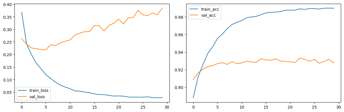
- 4. 모델 평가
model.eval()
test_loss = 0.0
test_total = 0
test_correct = 0

with torch.no_grad():
  for batch_idx, (images, labels) in enumerate(test_loader):
    images, labels = images.to(device), labels.to(device)
    outputs = model(images)
    loss = criterion(outputs, labels)

    test_loss += loss.detach().cpu().item()
    _, pred = torch.max(outputs.data, 1)
    test_total += labels.size(0)
    test_correct += (pred == labels).sum().detach().cpu().item()

test_loss /= len(test_loader)
test_acc = test_correct / test_total

print(f"Test 결과: {test_acc=:.4f} {test_loss=:.4f}")
- 5. 특성맵 시각화
sample_image = tr_images[1].squeeze()
plt.imshow(sample_image, cmap='gray')
plt.axis('off')
plt.show()
class FeatureExtractor:
    def __init__(self, model, layer_name):
        self.model = model
        self.layer_name = layer_name
        self.features = None

        layer = dict(model.named_modules())[layer_name]
        layer.register_forward_hook(self.hook)

    def hook(self, module, input, output):
        self.features = output

    def get_features(self, x):
        self.model.eval()
        with torch.no_grad():
            _ = self.model(x)
        return self.features

inputs = tr_images[1:2].to(device)

conv1_extractor = FeatureExtractor(model, 'conv1')
feature_maps = conv1_extractor.get_features(inputs)
print(feature_maps.shape)	# torch.Size([1, 32, 28, 28])

feature_maps_np = feature_maps.cpu().numpy()

fig, axs = plt.subplots(4, 8, figsize=(15, 8))

for i in range(4):
    for j in range(8):
        axs[i, j].imshow(feature_maps_np[0, i * 8 + j, :, :], cmap='viridis')
        axs[i, j].axis('off')
        axs[i, j].set_title(f"Filter {i * 8 + j}", fontsize=8)

plt.suptitle("1st Conv Layer's Feature Maps")
plt.tight_layout()
plt.show()
inputs = tr_images[1:2].to(device)

conv2_extractor = FeatureExtractor(model, 'conv2')
feature_maps = conv2_extractor.get_features(inputs)
print(feature_maps.shape)	# torch.Size([1, 64, 26, 26])

feature_maps_np = feature_maps.cpu().numpy()

fig, axs = plt.subplots(8, 8, figsize=(15, 8))

for i in range(8):
    for j in range(8):
        axs[i, j].imshow(feature_maps_np[0, i * 8 + j, :, :], cmap='viridis')
        axs[i, j].axis('off')
        axs[i, j].set_title(f"Filter {i * 8 + j}", fontsize=8)

plt.suptitle("2nd Conv Layer's Feature Maps")
plt.tight_layout()
plt.show()
실습 (Color Image CNN - CIFAR10, colab)
CNN: 컬러 CIFAR10 데이터셋 활
💧 MNIST와 거의 동일하며, 컬러 이미지라 픽셀 수가 변한 정도
https://www.cs.toronto.edu/~kriz/cifar.html
CIFAR-10 and CIFAR-100 datasets
< Back to Alex Krizhevsky's home page The CIFAR-10 and CIFAR-100 datasets are labeled subsets of the 80 million tiny images dataset. CIFAR-10 and CIFAR-100 were created by Alex Krizhevsky, Vinod Nair, and Geoffrey Hinton. The CIFAR-10 dataset The CIFAR-10
www.cs.toronto.edu
- 1. 데이터 로드
from torchvision.datasets import CIFAR10
from torchvision import transforms

transform = transforms.Compose([
    transforms.ToTensor(),
    transforms.Normalize((0.5, 0.5, 0.5), (0.5, 0.5, 0.5))  # 데이터 정규화 (RGB 평균, 표준편차)
])

trainset = CIFAR10(root='./', train=True, download=True, transform=transform)
testset = CIFAR10(root='./', train=False, download=True, transform=transform)
from torch.utils.data import DataLoader
batch_size = 64
train_loader = DataLoader(trainset, batch_size=batch_size, shuffle=True)
test_loader = DataLoader(testset, batch_size=batch_size, shuffle=False)
train_iter = iter(train_loader)
images, labels = next(train_iter)
print(images.shape)
print(labels.shape)
"""
torch.Size([64, 3, 32, 32]) # 3: 채널, 32: 가로, 32: 세로
torch.Size([64])
"""
first_image, first_label = images[0], labels[0]
print(first_image)
print(first_label)
print(trainset.classes)
"""
tensor([[[-0.6314, -0.5686, -0.6549, ..., -0.5373, -0.5137, -0.4745], # R
[-0.6471, -0.6078, -0.6235, ..., -0.5765, -0.5608, -0.5137],
[-0.6392, -0.6000, -0.6314, ..., -0.5686, -0.5686, -0.5608],
...,
[-0.6314, -0.6157, -0.6392, ..., -0.6863, -0.6314, -0.5765],
[-0.6392, -0.6549, -0.6863, ..., -0.6627, -0.6078, -0.5686],
[-0.4902, -0.4510, -0.4275, ..., -0.5608, -0.5451, -0.5451]],
[[-0.6314, -0.5765, -0.6627, ..., -0.3725, -0.3647, -0.3569], # G
[-0.6471, -0.6078, -0.6314, ..., -0.4353, -0.4196, -0.3804],
[-0.6392, -0.6078, -0.6392, ..., -0.4510, -0.4431, -0.4196],
...,
[-0.6392, -0.6471, -0.6941, ..., -0.7176, -0.6706, -0.6314],
[-0.6392, -0.6706, -0.7333, ..., -0.7098, -0.6627, -0.6235],
[-0.5059, -0.4902, -0.4902, ..., -0.6000, -0.5922, -0.5843]],
[[-0.5451, -0.4667, -0.5373, ..., -0.3647, -0.3569, -0.3333], # B
[-0.5686, -0.5059, -0.5137, ..., -0.4196, -0.4039, -0.3647],
[-0.5529, -0.4980, -0.5216, ..., -0.4275, -0.4275, -0.4039],
...,
[-0.5765, -0.5686, -0.6078, ..., -0.6000, -0.5608, -0.5529],
[-0.6000, -0.6314, -0.6314, ..., -0.6314, -0.5843, -0.5608],
[-0.4667, -0.4431, -0.3804, ..., -0.5529, -0.5373, -0.5294]]])
tensor(8)
['airplane', 'automobile', 'bird', 'cat', 'deer', 'dog', 'frog', 'horse', 'ship', 'truck']
"""
- 2. 데이터 시각화
import matplotlib.pyplot as plt
import torch

loader = DataLoader(trainset, batch_size=16, shuffle=True)
images, labels = next(iter(loader))

fig, axes = plt.subplots(1, 8, figsize=(22, 4))

for i in range(8):
    img = images[i].permute(1, 2, 0)
    img = (img * 0.5) + 0.5
    img = torch.clamp(img, 0, 1)	# 0과 1을 넘는 범위값들 정리
    axes[i].imshow(img.numpy())

    axes[i].set_title(trainset.classes[labels[i]])
    axes[i].axis('off')
plt.show()
- 3. 모델 생성
import torch.nn as nn
import torch.nn.functional as F
import torch.optim as optim

class CIFAR10_CNN(nn.Module):
    def __init__(self):
        super().__init__()

        # conv 블럭 1
        self.conv1_1 = nn.Conv2d(3, 32, kernel_size=3, padding=1)
        self.conv1_2 = nn.Conv2d(32, 32, kernel_size=3, padding=1)
        self.pool1 = nn.MaxPool2d(kernel_size=2, stride=2)      # 16*16

        # conv 블럭 2
        self.conv2_1 = nn.Conv2d(32, 64, kernel_size=3, padding=1)
        self.conv2_2 = nn.Conv2d(64, 64, kernel_size=3, padding=1)
        self.pool2 = nn.MaxPool2d(kernel_size=2, stride=2)      # 8*8

        # conv 블럭 3
        self.conv3_1 = nn.Conv2d(64, 128, kernel_size=3, padding=1)
        self.conv3_2 = nn.Conv2d(128, 128, kernel_size=3, padding=1)
        self.pool3 = nn.MaxPool2d(kernel_size=2, stride=2)      # 4*4

        # 완전연결층
        self.flatten = nn.Flatten()
        self.dropout1 = nn.Dropout(0.5)
        self.fc1 = nn.Linear(128 * 4 * 4, 300)
        self.dropout2 = nn.Dropout(0.3)
        self.fc2 = nn.Linear(300, 10)

    def forward(self, x):
        x = F.relu(self.conv1_1(x))
        x = F.relu(self.conv1_2(x))
        x = self.pool1(x)

        x = F.relu(self.conv2_1(x))
        x = F.relu(self.conv2_2(x))
        x = self.pool2(x)

        x = F.relu(self.conv3_1(x))
        x = F.relu(self.conv3_2(x))
        x = self.pool3(x)

        x = self.flatten(x)
        x = self.dropout1(x)
        x = F.relu(self.fc1(x))
        x = self.dropout2(x)
        return self.fc2(x)

model = CIFAR10_CNN()
print(model)
from torchsummary import summary
summary(model, (3, 32, 32), device='cpu')
"""
----------------------------------------------------------------
Layer (type) Output Shape Param #
================================================================
Conv2d-1 [-1, 32, 32, 32] 896
Conv2d-2 [-1, 32, 32, 32] 9,248
MaxPool2d-3 [-1, 32, 16, 16] 0
Conv2d-4 [-1, 64, 16, 16] 18,496
Conv2d-5 [-1, 64, 16, 16] 36,928
MaxPool2d-6 [-1, 64, 8, 8] 0
Conv2d-7 [-1, 128, 8, 8] 73,856
Conv2d-8 [-1, 128, 8, 8] 147,584
MaxPool2d-9 [-1, 128, 4, 4] 0
Flatten-10 [-1, 2048] 0
Dropout-11 [-1, 2048] 0
Linear-12 [-1, 300] 614,700
Dropout-13 [-1, 300] 0
Linear-14 [-1, 10] 3,010
================================================================
Total params: 904,718
Trainable params: 904,718
Non-trainable params: 0
----------------------------------------------------------------
Input size (MB): 0.01
Forward/backward pass size (MB): 1.02
Params size (MB): 3.45
Estimated Total Size (MB): 4.48
----------------------------------------------------------------
"""
- 4. 모델 학습
from torch.optim.lr_scheduler import ReduceLROnPlateau
from torch.utils.data import random_split

criterion = nn.CrossEntropyLoss()
optimizer = optim.Adam(model.parameters(), lr=0.001)

scheduler = ReduceLROnPlateau(optimizer, mode='min', factor=0.5, patience=3)

train_size = int(0.85 * len(trainset))
val_size = len(trainset) - train_size

train_dataset, val_dataset = random_split(trainset, [train_size, val_size])
train_loader = DataLoader(train_dataset, batch_size=batch_size, shuffle=True)
val_loader = DataLoader(val_dataset, batch_size=batch_size, shuffle=False)

device = torch.device('cuda' if torch.cuda.is_available() else 'cpu')
model = model.to(device)
from tqdm import tqdm
history = {
"train_loss": [],
"train_acc": [],
"val_loss": [],
"val_acc": []
}
epochs = 30
best_val_loss = float("inf")
patience = 5
patience_counter = 0
for epoch in tqdm(range(epochs)):
model.train()
train_loss = 0.0
train_total = 0
train_correct = 0
for batch_idx, (images, labels) in enumerate(train_loader):
images, labels = images.to(device), labels.to(device)
optimizer.zero_grad()
outputs = model(images)
loss = criterion(outputs, labels)
loss.backward()
optimizer.step()
train_loss += loss.detach().cpu().item()
_, pred = torch.max(outputs.data, 1)
train_total += labels.size(0)
train_correct += (pred == labels).sum().detach().cpu().item()
model.eval()
val_loss = 0.0
val_total = 0
val_correct = 0
with torch.no_grad():
for batch_idx, (images, labels) in enumerate(val_loader):
images, labels = images.to(device), labels.to(device)
outputs = model(images)
loss = criterion(outputs, labels)
val_loss += loss.detach().cpu().item()
_, pred = torch.max(outputs.data, 1)
val_total += labels.size(0)
val_correct += (pred == labels).sum().detach().cpu().item()
train_loss /= len(train_loader)
val_loss /= len(val_loader)
train_acc = train_correct / train_total
val_acc = val_correct / val_total
history["train_loss"].append(train_loss)
history["train_acc"].append(train_acc)
history["val_loss"].append(val_loss)
history["val_acc"].append(val_acc)
if (epoch + 1) % 5 == 0:
print(f"Epoch [{epoch + 1}/{epochs}] {train_acc=:.4f} {train_loss=:.4f} {val_acc=:.4f} {val_loss=:.4f}")
scheduler.step(val_loss)
if val_loss < best_val_loss:
best_val_loss = val_loss
patience_counter = 0
else:
patience_counter += 1
if patience_counter >= patience:
print(f"조기 종료 ... epoch: {epoch + 1}")
break# 학습 시각화
plt.figure(figsize=(12, 4))
plt.subplot(1, 2, 1)
plt.plot(history['train_loss'], label='train_loss')
plt.plot(history['val_loss'], label='val_loss')
plt.legend()
plt.subplot(1, 2, 2)
plt.plot(history['train_acc'], label='train_acc')
plt.plot(history['val_acc'], label='val_acc')
plt.legend()
plt.tight_layout()
plt.show()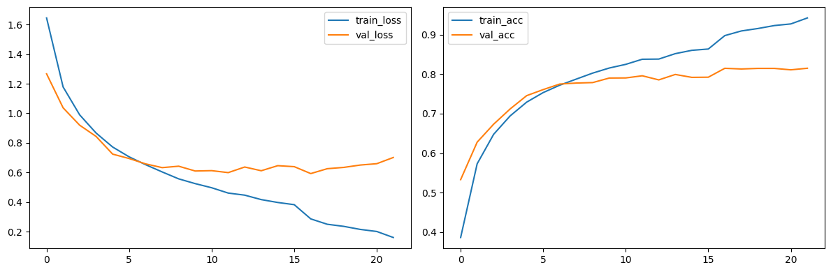
- 5. 모델 평가
model.eval()
test_loss = 0.0
test_total = 0
test_correct = 0

with torch.no_grad():
    for batch_idx, (images, labels) in enumerate(test_loader):
        images, labels = images.to(device), labels.to(device)
        outputs = model(images)
        loss = criterion(outputs, labels)

        test_loss += loss.detach().cpu().item()
        _, pred = torch.max(outputs.data, 1)
        test_total += labels.size(0)
        test_correct += (pred == labels).sum().detach().cpu().item()

test_loss /= len(test_loader)
test_acc = test_correct / test_total

print(f"Test 결과: {test_acc=:.4f} {test_loss=:.4f}")
# Test 결과: test_acc=0.8143 test_loss=0.7483
'LLM' 카테고리의 다른 글
| 3.3.23 [LLM] 자연어-이미지 멀티모달: 이미지 딥러닝 응용(스타일 전이 학습, GAN) (1) | 2025.09.28 |
|---|---|
| 3.3.22 [LLM] 자연어-이미지 멀티모달: 주요 CNN 모델 (0) | 2025.09.28 |
| 3.3.20 [LLM] 자연어-이미지 멀티모달: etc (0) | 2025.09.15 |
| 3.3.19 [LLM] 파인튜닝 기법: DPO (0) | 2025.09.15 |
| 3.3.18 [LLM] 파인튜닝 기법: RLHF (0) | 2025.09.14 |
